エクセルのグラフで系列の参照範囲を変更する

2021-09-09

エクセルのグラフで参照範囲を変更する方法です。

グラフ参照範囲変更例

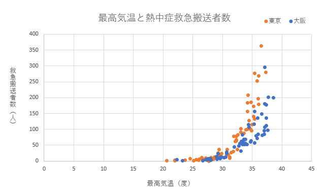
1日の最高気温と熱中症救急搬送者数の散布図の例です。

グラフとデータ

作成後のグラフです。

参考：気温が上がると熱中症の救急搬送者数が増える関係がわかります。

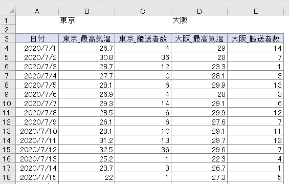
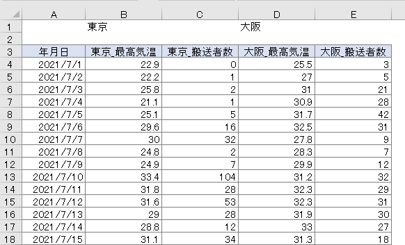
グラフのもとになるデータです。

東京と大阪の1日の最高気温と熱中症救急搬送者数のデータです。

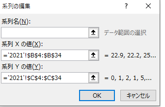
例えば違う年のデータにグラフをコピーした場合、グラフをコピーすると参照範囲が違います。この参照範囲をマクロで変更します。

データについて

気温：気象庁
出典：気象庁ホームページ（https://www.jma.go.jp/）
救急搬送者数：総務省消防庁
出典：消防庁ホームページ（http://www.fdma.go.jp/）

サンプルコード

変更するグラフを選択した状態でマクロを実行します。

Sub sample()
    Dim i As Long, r As Long, c As Long
    Dim sc As Series
    Dim lastR As Long
    
    i = 1
    r = 4
    For c = 2 To 4 Step 2
        Set sc = ActiveChart.SeriesCollection(i)
        lastR = Cells(Rows.Count, c).End(xlUp).Row
        With sc
            .Name = Cells(1, c)
            .XValues = Range(Cells(r, c), Cells(lastR, c))
            .Values = Range(Cells(r, c + 1), Cells(lastR, c + 1))
        End With
        i = i + 1
    Next c
End Sub

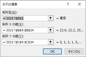
この例では系列名が参照されていません。

系列名を参照にする場合

Sub sample2()
    Dim i As Long, r As Long, c As Long
    Dim sc As Series
    Dim lastR As Long
    Dim ws As String: ws = ActiveSheet.Name
    
    i = 1
    r = 4
    For c = 2 To 4 Step 2
        Set sc = ActiveChart.SeriesCollection(i)
        lastR = Cells(Rows.Count, c).End(xlUp).Row
        With sc
            .Name = "='" & ws & "'!R1C" & c
            .XValues = Range(Cells(r, c), Cells(lastR, c))
            .Values = Range(Cells(r, c + 1), Cells(lastR, c + 1))
        End With
        i = i + 1
    Next c
End Sub